


FFT Zero Padding
The Fast Fourier Transform (FFT) is one of the most used tools in electrical engineering analysis, but certain aspects of the transform are not widely understood–even by engineers who think they understand the FFT. Some of the most commonly misunderstood concepts are zero-padding, frequency resolution, and how to choose the right Fourier transform size.
This article will explore zero-padding the Fourier transform–how to do it correctly and what is actually happening. The exploration will cover of the following topics:
- Zero Padding
- FFT Frequency Resolution
- Waveform Frequency Resolution
- FFT Resolution
- Frequency Domain Resolution Concept Exploration
- Choosing the Right FFT Size.
Zero Padding
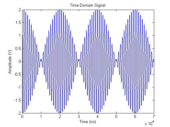
Zero padding is a simple concept; it simply refers to adding zeros to end of a time-domain signal to increase its length. The example 1 MHz and 1.05 MHz real-valued sinusoid waveforms we will be using throughout this article is shown in the following plot:
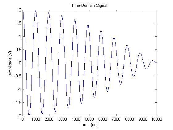
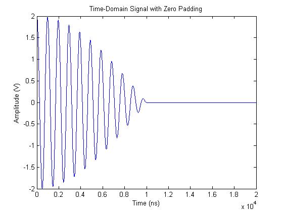
The time-domain length of this waveform is 1000 samples. At the sampling rate of 100 MHz, that is a time-length of 10 us. If we zero pad the waveform with an additional 1000 samples (or 10 us of data), the resulting waveform is produced:
There are a few reasons why you might want to zero pad time-domain data. The most common reason is to make a waveform have a power-of-two number of samples. When the time-domain length of a waveform is a power of two, radix-2 FFT algorithms, which are extremely efficient, can be used to speed up processing time. FFT algorithms made for FPGAs also typically only work on lengths of power two.
While it’s often necessary to stick to powers of two in your time-domain waveform length, it’s important to keep in mind how doing that affects the resolution of your frequency-domain output.
FFT Frequency Resolution
There are two aspects of FFT resolution. I’ll call the first one “waveform frequency resolution” and the second one “FFT resolution”. These are not technical names, but I find them helpful for the sake of this discussion. The two can often be confused because when the signal is not zero padded, the two resolutions are equivalent.
The “waveform frequency resolution” is the minimum spacing between two frequencies that can be resolved. The “FFT resolution” is the number of points in the spectrum, which is directly proportional to the number points used in the FFT.
It is possible to have extremely fine FFT resolution, yet not be able to resolve two coarsely separated frequencies.
It is also possible to have fine waveform frequency resolution, but have the peak energy of the sinusoid spread throughout the entire spectrum (this is called FFT spectral leakage).
The waveform frequency resolution is defined by the following equation:

where T is the time length of the signal with data. It’s important to note here that you should not include any zero padding in this time! Only consider the actual data samples.
It’s important to make the connection here that the discrete time Fourier transform (DTFT) or FFT operates on the data as if it were an infinite sequence with zeros on either side of the waveform. This is why the FFT has the distinctive sinc function shape at each frequency bin.
You should recognize the waveform resolution equation 1/T is the same as the space between nulls of a sinc function.
The FFT resolution is defined by the following equation:
Frequency Domain Resolution Concept Exploration
Considering our example waveform with 1 V-peak sinusoids at 1 MHz and 1.05 MHz, let’s start exploring these concepts.
Let’s start off by thinking about what we should expect to see in a power spectrum. Since both sinusoids have 1 Vpeak amplitudes, we should expect to see spikes in the frequency domain with 10 dBm amplitude at both 1 MHz and 1.05 MHz.
The original time-domain signal shown in the first plot with a length of 1000 samples (10 us). A 1000-point FFT used on the time-domain signal is shown in the next figure:

Two distinct peaks are not shown, and the single wide peak has an amplitude of about 11.4 dBm. Clearly these results don’t give an accurate picture of the spectrum. There is not enough resolution in the frequency domain to see both peaks.
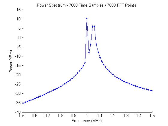
Let’s try to resolve the two peaks in the frequency domain by using a larger FFT, thus adding more points to the spectrum along the frequency axis. Let’s use a 7000-point FFT. This is done by zero padding the time-domain signal with 6000 zeros (60 us). The zero-padded time-domain signal is shown here:
The resulting frequency-domain data, shown as a power spectrum, is shown here:

Although we’ve added many more frequency points, we still cannot resolve the two sinuoids; we are also still not getting the expected power.
Taking a closer look at what this plot is telling us, we see that all we have done by adding more FFT points is to more clearly define the underlying sinc function arising from the waveform frequency resolution equation. You can see that the sinc nulls are spaced at about 0.1 MHz.
Because our two sinusoids are spaced only 0.05 MHz apart, no matter how many FFT points (zero padding) we use, we will never be able to resolve the two sinusoids.
Let’s look at what the resolution equations are telling us. Although the FFT resolution is about 14 kHz (more than enough resoution), the waveform frequency resolution is only 100 kHz. The spacing between signals is 50 kHz, so we are being limited by the waveform frequency resolution.
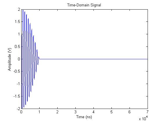
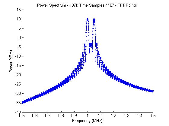
To resolve the spectrum properly, we need to increase the amount of time-domain data we are using. Instead of zero padding the signal out to 70 us (7000 points), let’s capture 7000 points of the waveform. The time-domain and domain results are shown here, respectively.
The resulting frequency-domain data, shown as a power spectrum, is shown here:
With the expanded time-domain data, the waveform frequency resolution is now about 14 kHz as well. As seen in the power spectrum plot, the two sinusoids are not seen. The 1 MHz signal is clearly represented and is at the correct power level of 10 dBm, but the 1.05 MHz signal is wider and not showing the expected power level of 10 dBm. What gives?
What is happening with the 1.05 MHz signal is that we don’t have an FFT point at 1.05 MHz, so the energy is split between multiple FFT bins.
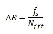
The spacing between FFT points follows the equation:
where nfft is the number of FFT points and fs is the sampling frequency.
In our example, we’re using a sampling frequency of 100 MHz and a 7000-point FFT. This gives us a spacing between points of 14.28 kHz. The frequency of 1 MHz is a multiple of the spacing, but 1.05 MHz is not. The closest frequencies to 1.05 MHz are 1.043 MHz 1.057 MHz, so the energy is split between the two FFT bins.
To solve this issue, we can choose the FFT size so that both frequencies are single points along the frequency axis. Since we don’t need finer waveform frequency resolution, it’s okay to just zero pad the time-domain data to adjust the FFT point spacing.
Adding an additional 1000 zeros (10 us) to the time-domain signal gives us a spacing of 12.5 kHz, and both 1 MHz and 1.05 MHz are integer multiples of the spacing. The resulting spectrum is shown in the following figure.
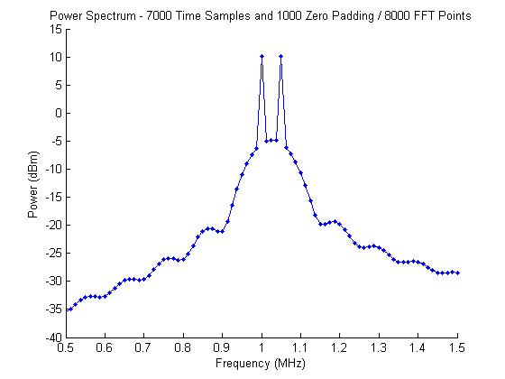
Now both frequencies are resolved and at the expected power of 10 dBm.
For the sake of overkill, you can always add more points to your FFT through zero padding (ensuring that you have the correct waveform resolution) to see the shape of the FFT bins as well. This is shown in the following figure:
Choosing the Right FFT Size
Three considerations should factor into your choice of FFT size, zero padding, and time-domain data length.
- What waveform frequency resolution do you need?
- What FFT resolution do you need?
- Does your choice of FFT size allow you to inspect particular frequencies of interest?
1) The waveform frequency resolution should be smaller than the minimum spacing between frequencies of interest.
2) The FFT resolution should at least support the same resolution as your waveform frequency resolution. Additionally, some highly-efficient implementations of the FFT require that the number of FFT points be a power of two.
3) You should ensure that there are enough points in the FFT, or the FFT has the correct spacing set, so that your frequencies of interest are not split between multiple FFT points.
One final thought on zero padding the FFT:
If you apply a windowing function to your waveform, the windowing function needs to be applied before zero padding the data. This ensures that your real waveform data starts and ends at zero, which is the point of most windowing functions.
Thanks for reading!
We want to hear from you! Do you have a comment, question, or suggestion? Twitter us @bitweenie or me @shilbertbw, or leave a comment right here!
Recent Comments